Query profiling

Monitor query execution across workers to identify bottlenecks, understand data flow, and optimize performance.

Types of operations in a query

To optimize a query it helps to understand where it spends its time. Each worker in a distributed query does three things: it reads data, computes on it, and exchanges data with other workers.

Input/Output: Each worker reads its assigned partitions from storage and writes results to a destination. These are typically the first and last activities you see in the profiler. I/O-heavy queries benefit from more network bandwidth, either by adding more nodes or by choosing a higher-bandwidth instance type.

Computation: Workers execute the query operations (such as filters, joins, aggregations, etc.) on their local data. CPU and memory usage are visible in the resource overview of the nodes.

Shuffling: Some operations, such as joins and group-bys, require all rows with a given key to be on the same worker. To accomplish this, data is redistributed across the cluster in a shuffle between stages. Within a stage, the streaming engine processes incoming shuffle data as it arrives over the network, so I/O and computation overlap. Shuffle-heavy queries produce large volumes of inter-node traffic, visible as network bandwidth usage in the cluster dashboard and as a high percentage of time spent shuffling in the metrics.

Using the query profiler

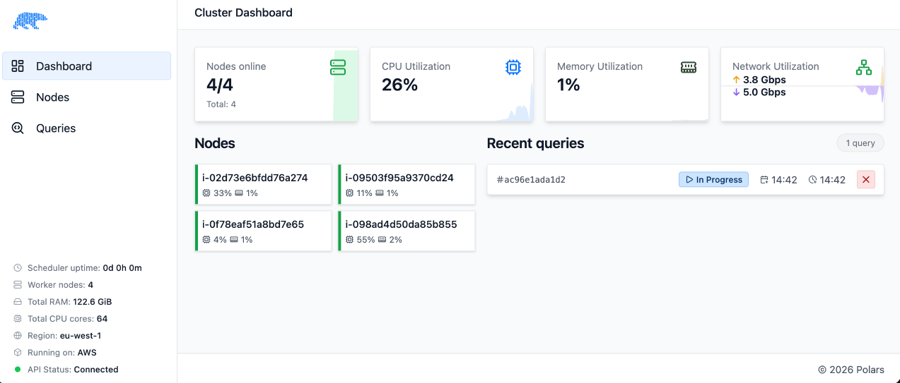
The cluster dashboard and built-in query profiler are available through the Polars Cloud compute dashboard.

The profiler shows detailed metrics, both real-time and after query completion, such as workers' resource usage and the percentage of time spent shuffling.

Single Node Query

Our first example is a query that runs on a single node. If you'd like you can run this in your own environment so you can explore the functionality yourself.

Try it: Single node query

Queries can be run on a single node by marking your query like so:

query.remote(ctx).single_node().execute()

This will let the query run on a single worker. This simplifies query execution and you don't need to shuffle data between workers. Copy and paste the example below to explore the feature yourself. Don't forget to change the workspace name to one of your own workspaces.

Python

import polars as pl
import polars_cloud as pc
from datetime import date


pc.authenticate()
ctx = pc.ComputeContext(workspace="your-workspace", cpus=8, memory=8, cluster_size=1)

lineitem = pl.scan_parquet("s3://polars-cloud-samples-us-east-2-prd/pdsh/sf10/lineitem.parquet",
    storage_options={"request_payer": "true"}
)
var1 = date(1998, 9, 2)

(
    lineitem.filter(pl.col("l_shipdate") <= var1)
    .group_by("l_returnflag", "l_linestatus")
    .agg(
        pl.sum("l_quantity").alias("sum_qty"),
        pl.sum("l_extendedprice").alias("sum_base_price"),
        (pl.col("l_extendedprice") * (1.0 - pl.col("l_discount")))
        .sum()
        .alias("sum_disc_price"),
        (
            pl.col("l_extendedprice")
            * (1.0 - pl.col("l_discount"))
            * (1.0 + pl.col("l_tax"))
        )
        .sum()
        .alias("sum_charge"),
        pl.mean("l_quantity").alias("avg_qty"),
        pl.mean("l_extendedprice").alias("avg_price"),
        pl.mean("l_discount").alias("avg_disc"),
        pl.len().alias("count_order"),
    )
    .sort("l_returnflag", "l_linestatus")
).remote(ctx).single_node().execute()

Query plans

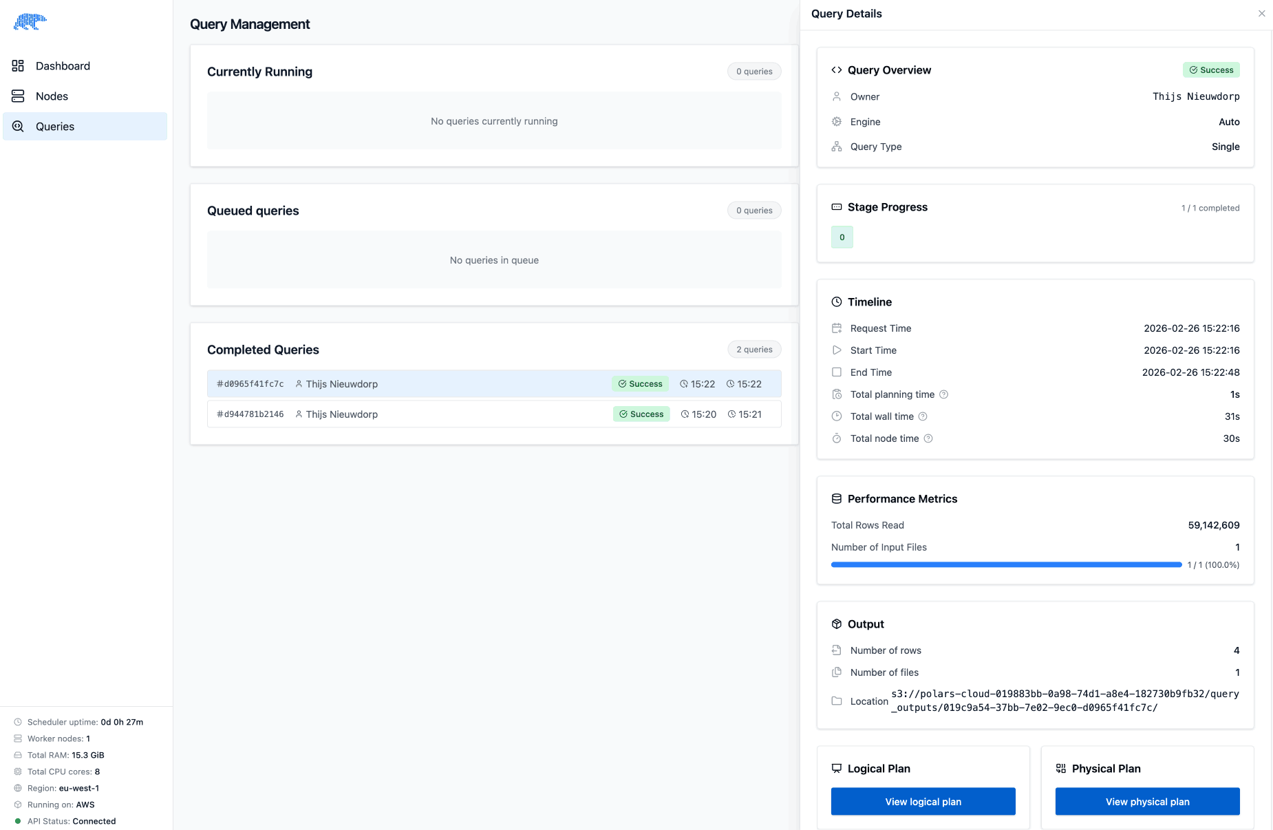
You can inspect the details of a query by going to the "Queries" tab and selecting the query you want to inspect. You can see the timeline, which shows when the query started and ended, and how long planning and running the query took. On top of that it consists of a single stage, because the query runs completely on a single node.

At the bottom of the query details you can inspect the optimized logical plan and the physical plan:

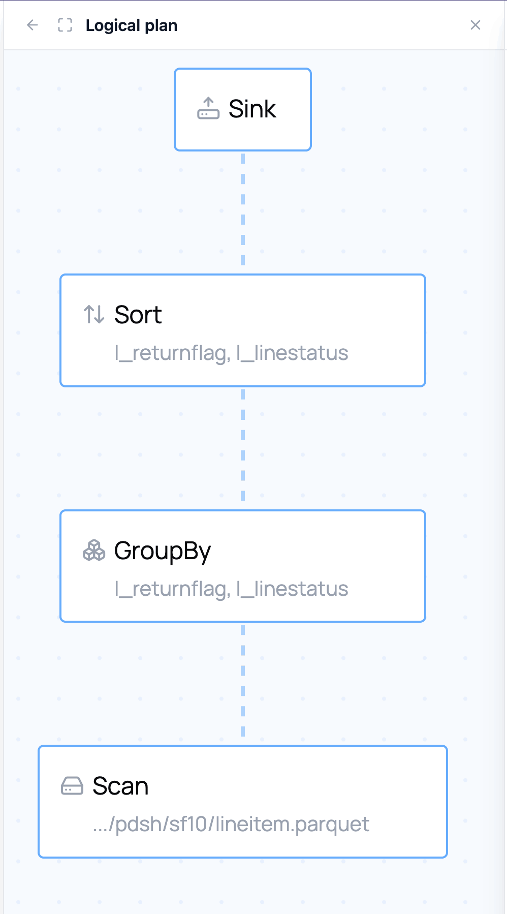
The logical plan is a graph representation that shows what your query will do, and how your query has been optimized. Clicking nodes in the plan gives you more details about the operation that will be performed:

The physical plan shows how the engine executes your query: the concrete algorithms, operator implementations, and data flow chosen at runtime.

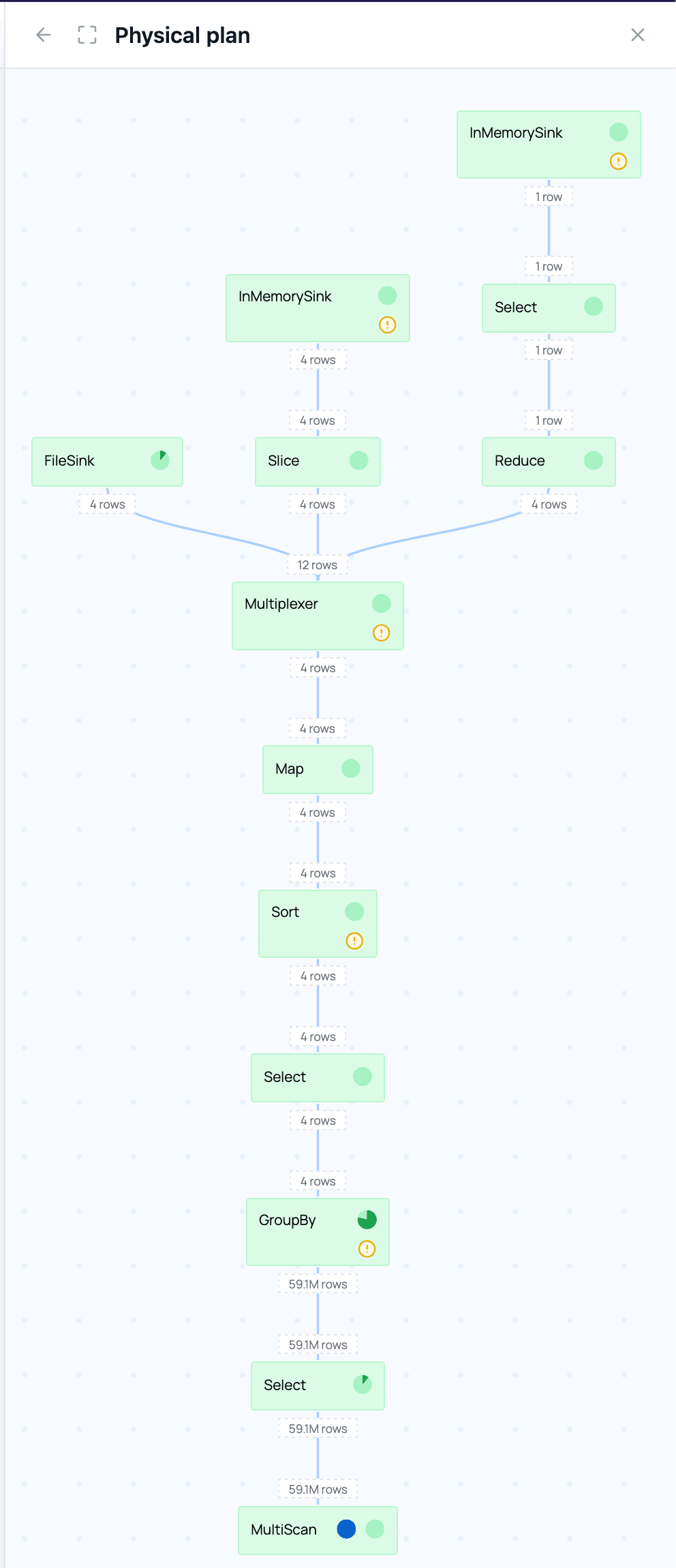
While the query runs and after it has finished, there are additional metrics available, such as how many rows and morsels flow through a node and how much time is spent in that node. In our example you can see that the group by takes particularly long and aggregates an input of 59.1 million rows to 4 output rows:

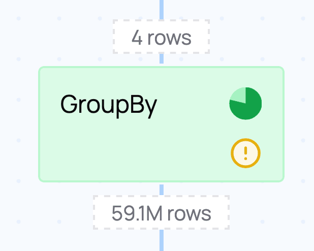
This makes sense because this query performs a list of aggregations, as we can see in the node details information in the logical plan:

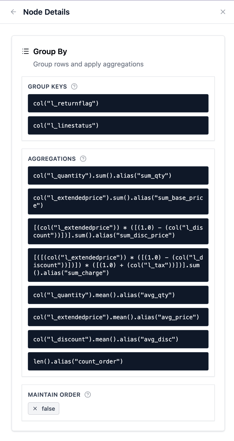
The indication that most time is spent in the GroupBy node matches our expectations for this query.

Indicators

Modes in the physical plan or stages in the stage graph can show indicators to help identify bottlenecks:

Indicator	Description
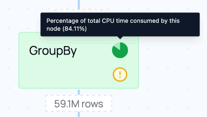	Shows which operations took the most CPU time.
	Percentage of the stage's total I/O time spent in this node, helping identify the most I/O-heavy operations.
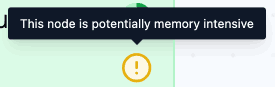	The node is potentially memory-intensive because the operation requires keeping state (e.g. storing the intermediate groups in a group_by).
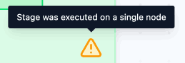	This stage was executed on a single node because it contains operations that require a global state (e.g. sort). This indicator only appears in distributed queries.
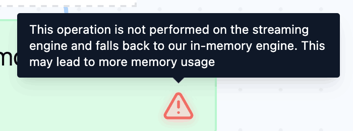	This operation is currently not supported on the streaming engine and was executed on the in-memory engine.

I/O and CPU time don't sum to 100%

The I/O time and CPU time percentages shown per node do not sum to the total runtime. This is because execution is pipelined: data is processed as it arrives, so I/O (reading/writing) and CPU (computation) work happens concurrently. As a result, both indicators can be non-zero at the same time for a given node, and their combined total can exceed the total runtime.

Distributed Query

The following section is based on a distributed query. You can follow along with this example code:

Try it: Distributed query

Distributed is the default execution mode in Polars Cloud. You can also set it explicitly:

query.remote(ctx).distributed().execute()

For more on how distributed execution works, see Distributed queries. Copy and paste the example below to explore the feature yourself. Don't forget to change the workspace name to one of your own workspaces.

Python

import polars as pl
import polars_cloud as pc

pc.authenticate()

ctx = pc.ComputeContext(workspace="your-workspace", cpus=12, memory=12, cluster_size=4)

def pdsh_q3(customer, lineitem, orders):
    return (
        customer.filter(pl.col("c_mktsegment") == "BUILDING")
        .join(orders, left_on="c_custkey", right_on="o_custkey")
        .join(lineitem, left_on="o_orderkey", right_on="l_orderkey")
        .filter(pl.col("o_orderdate") < pl.date(1995, 3, 15))
        .filter(pl.col("l_shipdate") > pl.date(1995, 3, 15))
        .with_columns(
            (pl.col("l_extendedprice") * (1 - pl.col("l_discount"))).alias("revenue")
        )
        .group_by("o_orderkey", "o_orderdate", "o_shippriority")
        .agg(pl.sum("revenue"))
        .select(
            pl.col("o_orderkey").alias("l_orderkey"),
            "revenue",
            "o_orderdate",
            "o_shippriority",
        )
        .sort(by=["revenue", "o_orderdate"], descending=[True, False])
    )

lineitem = pl.scan_parquet(
    "s3://polars-cloud-samples-us-east-2-prd/pdsh/sf100/lineitem/*.parquet",
    storage_options={"request_payer": "true"},
)
customer = pl.scan_parquet(
    "s3://polars-cloud-samples-us-east-2-prd/pdsh/sf100/customer/*.parquet",
    storage_options={"request_payer": "true"},
)
orders = pl.scan_parquet(
    "s3://polars-cloud-samples-us-east-2-prd/pdsh/sf100/orders/*.parquet",
    storage_options={"request_payer": "true"},
)

pdsh_q3(customer, lineitem, orders).remote(ctx).distributed().execute()

Stage graph

When executing distributed queries, queries are often executed in stages. Some operations require shuffles to make sure the correct partitions are available to the workers. To accomplish this, data is shuffled between workers over the network. Each stage can be expanded to inspect the operations it contains and understand what work is happening at each point in the pipeline.

When you execute the example query, you get the result that can be seen in the image below. In the stage graph, one of the scan stages at the bottom stands out: its indicator shows a high percentage of total time spent in that stage.

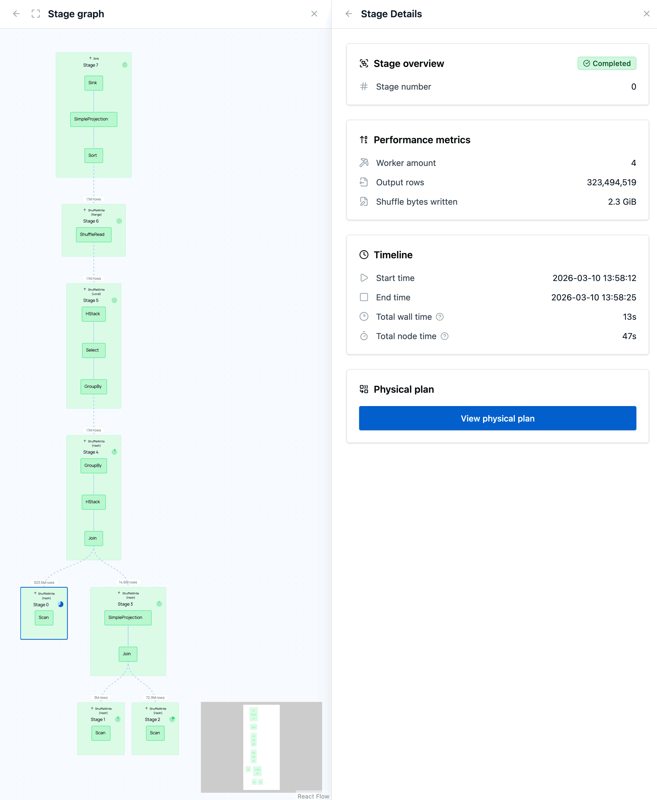
When you click on that stage (not one of the nodes in it), you open the stage details, displaying detailed metrics. You can notice that the I/O time of this stage is roughly 55%.

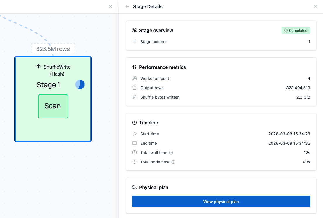
Through the details you can open the physical plan of this stage. This will display all of the operations in this stage, how long they took, and any indicators that might help you find bottlenecks.

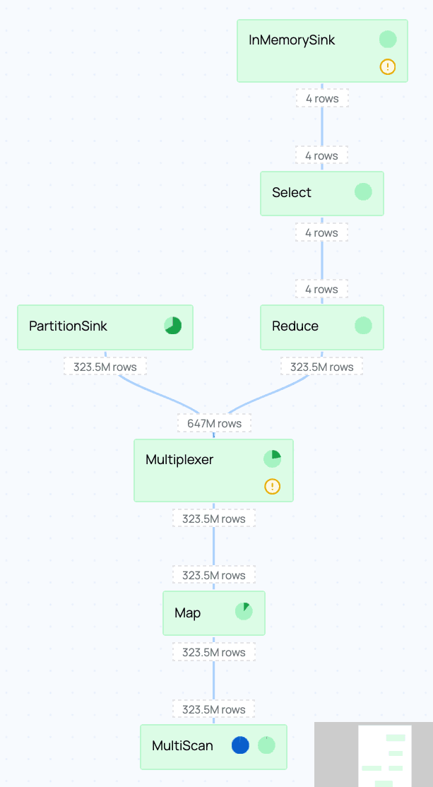
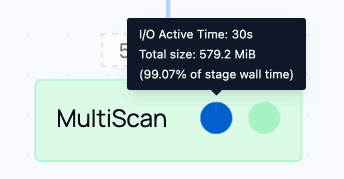
One thing you should immediately notice is that the MultiScan node at the bottom takes almost 100% of the time for I/O:

This I/O indicator shows that I/O was active for nearly the full runtime of the stage. We can conclude that the network I/O in this node is the bottleneck in this part of the physical plan.

In this example the data is stored in us-east-2 while the cluster runs in eu-west-1. The cross-region bandwidth causes I/O to take longer than it would if the data and cluster were in the same region. Co-locate your cluster and data in the same region to minimize I/O latency.

Takeaways

• The logical plan shows how your query has been optimized.
• The physical plan shows how your query is executed, and which operations are responsible for both CPU and I/O time spent.
• In a distributed query, the stage graph shows which stages take the longest and how much data is shuffled between them.
• Indicators on stages and nodes highlight potential bottlenecks: start with the slowest stage and drill down to individual operations.
• I/O-heavy queries benefit from more bandwidth: you can add nodes or choose a higher-bandwidth instance type.
• Shuffle-heavy queries may benefit from fewer, larger nodes to reduce inter-node traffic.