Distributed queries

With the introduction of Polars Cloud, we also introduced the distributed engine. This engine enables users to horizontally scale workloads across multiple machines.

Polars has always been optimized for fast and efficient performance on a single machine. However, when querying large datasets from cloud storage, performance is often constrained by the I/O limitations of a single node. By scaling horizontally, these download limitations can be significantly reduced, allowing users to process data at scale.

Distributed engine is in open beta

The distributed engine currently supports most of Polars API and datatypes. Follow the tracking issue to stay up to date.

Using distributed engine

To execute queries using the distributed engine, you can call the distributed() method. This is the default mode of execution for remote queries.

lf: LazyFrame

result = (
      lf.remote()
      .distributed()
      .execute()
)

Example

This example demonstrates running query 3 of the PDS-H benchmarkon scale factor 100 (approx. 100GB of data) using Polars Cloud distributed engine.

Run the example yourself

Copy and paste the code to you environment and run it. The data is hosted in S3 buckets that use AWS Requester Pays, meaning you pay only for pays the cost of the request and the data download from the bucket. The storage costs are covered.

First import the required packages and point to the S3 bucket. In this example, we take one of the PDS-H benchmarks queries for demonstration purposes.

Python

import polars as pl
import polars_cloud as pc

lineitem_sf100 = pl.scan_parquet(
    "s3://polars-cloud-samples-us-east-2-prd/pdsh/sf100/lineitem/*.parquet",
    storage_options={"request_payer": "true"},
)
customer_sf100 = pl.scan_parquet(
    "s3://polars-cloud-samples-us-east-2-prd/pdsh/sf100/customer/*.parquet",
    storage_options={"request_payer": "true"},
)
orders_sf100 = pl.scan_parquet(
    "s3://polars-cloud-samples-us-east-2-prd/pdsh/sf100/orders/*.parquet",
    storage_options={"request_payer": "true"},
)

After that we define the query. Note that this query will also run on your local machine if you have the data available. You can generate the data with the Polars Benchmark repository.

Python

def pdsh_q3(
    customer: pl.LazyFrame, lineitem: pl.LazyFrame, orders: pl.LazyFrame
) -> pl.LazyFrame:
    return (
        customer.filter(pl.col("c_mktsegment") == "BUILDING")
        .join(orders, left_on="c_custkey", right_on="o_custkey")
        .join(lineitem, left_on="o_orderkey", right_on="l_orderkey")
        .filter(pl.col("o_orderdate") < pl.date(1995, 3, 15))
        .filter(pl.col("l_shipdate") > pl.date(1995, 3, 15))
        .with_columns(
            (pl.col("l_extendedprice") * (1 - pl.col("l_discount"))).alias("revenue")
        )
        .group_by("o_orderkey", "o_orderdate", "o_shippriority")
        .agg(pl.sum("revenue"))
        .select(
            pl.col("o_orderkey").alias("l_orderkey"),
            "revenue",
            "o_orderdate",
            "o_shippriority",
        )
        .sort(by=["revenue", "o_orderdate"], descending=[True, False])
    )

The final step is to set the compute context and run the query. Here we're using 5 nodes with 10 CPUs and 10GB memory each. Show() will return the first 10 rows back to your environment. The query takes around xx seconds to execute.

Python

ctx = pc.ComputeContext(workspace="your-workspace", cpus=4, memory=4, cluster_size=5)

pdsh_q3(customer_sf100, lineitem_sf100, orders_sf100).remote(ctx).distributed().show()

Try on SF1000 (approx. 1TB of data)

You can also run this example on a higher scale factor. The data is available on the same bucket. You can change the URL from sf100 to sf1000.

How it works

When you call .execute() on a distributed query, it passes through the following pipeline:

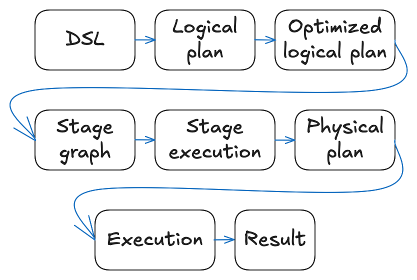
1. You write a query using the Polars DSL, building up a LazyFrame.
2. The LazyFrame is translated into a logical plan: a tree of operations capturing what to compute. You can inspect this logical plan by running lf.explain(optimized=False).
3. The query optimizer rewrites the logical plan into an equivalent but more efficient optimized logical plan. You can inspect the optimized logical plan with lf.explain().
4. The distributed query planner walks the optimized logical plan and produces a stage graph: a DAG of stages separated by shuffles at each point where a data needs to be redistributed across workers.
5. The scheduler executes stages and assigns partitions to workers in dependency order, waiting for all workers to finish before starting the next stage.
6. Each worker receives the optimized logical plan together with its assigned partitions, derives its own physical plan, and executes it. After finishing the stage, intermediate results are written to a local or network-shared disk.
7. After the final stage, results are written to the destination location, or sent back to the user, depending on the query.